
Two pharmaceutical loads leave the same regional distribution center for the same hospital network. Both carry temperature-sensitive biologics valued near $280,000. Both are monitored by the same device at the same per-trip cost.
Shipment A moves in July, through a corridor where ambient temperatures plausibly exceed 35 °C at a customs yard with an assumed average dwell of 14 hours. These figures are consistent with published summer thermal profiles for subtropical border crossings; they construct a contrast, not a measured route. Shipment B travels the same route in February, with ambient temperatures between 2 °C and 8 °C and a 20-minute dwell window.
The device cost is identical. The baseline excursion risk is not. The probability that an alert reaches a decision-maker who can divert, hold, or re-ice the load — the intervention capability — may also differ by season. Staffing levels, carrier contracts, and customs schedules all shift between summer and winter corridors. The economic return of monitoring these two loads is not the same number.
But the procurement model treats it as one, because the ranking key it uses is unit price per device, and that number is identical for both. The assumption being audited here is specific: the cheapest tracker that meets compliance specifications maximizes monitoring ROI.
Industry estimates place annual cold-chain product losses between $20 billion and $35 billion globally. No widely referenced source specifies the scope, methodology, or year in a way that survives independent audit. Cargo values on a single refrigerated trailer in pharmaceutical distribution can range from $50,000 to beyond $500,000. These are cargo values, not realized losses. Expected excursion probability, product stability, and addressable intervention all mediate what any fleet actually stands to recover.
The seven sections that follow test the unit-price ranking assumption against the economic structure it claims to describe.
Why This Ranking Rule Persists
Procurement systems are designed to score items with SKUs. Temperature monitoring devices have SKUs. Transportation lanes do not. When a logistics director submits a monitoring budget, the line item is hardware — a device cost multiplied by expected shipments. The return against that expenditure shows up months later as an exception report: loads that experienced excursions, products rejected, claims filed.
This separation is structural, not negligent. Capital expenditure approvals move through one workflow. Exception-cost recovery moves through another. The organization that approves the device purchase rarely sees cell-level loss data in the same view, at the same time, within the same decision model.
Unit price becomes the ranking key by default — not because anyone explicitly defends it as the correct unit of economics, but because it is the only metric that lives natively in the procurement system. Expected loss by shipment cell, addressable intervention value, and full program cost are all calculable. They require data from operations, quality, regulatory, and finance. That data integration is expensive. The device price is on the quote.
Three reinforcing mechanisms keep the ranking rule in place. First, vendor comparison sheets sort by unit price as the leftmost column. Second, volume discount structures reward commitment before risk segmentation has been performed. Third, pilot programs test a device on a convenience sample of routes rather than the routes where monitoring value is highest. The results are then averaged across the sample as though the cells were interchangeable.
The Unit-of-Analysis Error
The procurement assumption treats ROI as a property of the monitoring device — something that can be scored on a datasheet. That is the first error. Replacing "device" with "lane" is the second. A geographic corridor is still an over-aggregation: lane risk is not a single number. Two shipments on the same lane can differ materially in product value, packaging thermal mass, carrier service level, regulatory consequence, and intervention coverage.
The Shipment Cell
The economic unit that determines monitoring return is a shipment cell — defined by the combination of lane, product (including value and stability profile), packout, season, carrier and service mode, and response model. Two cells sharing the same origin and destination can produce different returns if any of these attributes changes. A July shipment of biologics in passive packaging through a border crossing with 14-hour dwell is not the same cell as a February shipment of the same product in active containers through the same crossing with a 20-minute dwell.
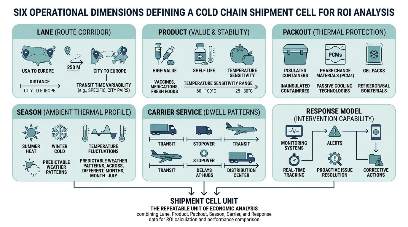
ROI belongs to a monitoring intervention applied to a shipment cell — measured against a current operational baseline. Unit price is one cost term in the denominator. It is not the object of return, and it is not a device attribute.
Same device, different cell, different return. What changes across cells is the baseline risk, the addressable fraction of that risk, and the full cost of acting on alerts — not the device's technical performance.
Device-level ROI scorecards — the kind that assign an ROI percentage to a tracker model based on its specifications — describe nothing a director can allocate budget against. Two monitoring programs applied to the same cell with the same device can also produce different returns. Alert thresholds, response protocols, escalation paths, and labor allocation all shape the outcome. ROI is an attribute of the intervention–cell pairing, not of the device, and not of the lane.
What Is at Stake When a Shipment Cell Fails
Loss estimates in the cold chain are widely cited but poorly sourced. The most common industry figure — annual global losses between $20 billion and $35 billion — appears across trade publications and vendor marketing. No version consistently attributes the estimate to a single study, year, or methodology. What the figure does establish, even imprecisely, is that the stakes are non-trivial and that they are not uniformly distributed.
Cargo values per load vary by at least an order of magnitude across segments. A $50,000 produce shipment and a $480,000 biologics load face different economic consequences from the same 4 °C excursion. But cargo value is not realized loss. A high-value load that experiences a brief excursion within its product stability budget may be released without consequence. A lower-value load that sits for 16 hours above its critical temperature at a transload facility may be a total write-off.
The relationship between exposure and loss is mediated by product tolerance, excursion duration and severity, packaging performance, and regulatory classification. Industry reports have described up to 25 % of certain pharmaceutical product categories as temperature-compromised during distribution. The definition of "compromised" varies by source — exposed to out-of-specification conditions, suspected of degradation, rejected at receipt, or actually rendered unusable — and each definition carries a materially different economic implication.
More importantly, not all loss is addressable by monitoring. Addressable value requires a causal chain: the device detects the excursion, the alert reaches a decision-maker in time, the decision-maker has an available intervention — divert, re-ice, hold, reject — and the intervention is effective. Where that chain breaks, monitoring produces evidence value — compliance records, claims documentation, carrier scorecards — but not avoided product loss. Those are different return paths with different economics.
Six Procurement Assumptions and Their Corrections
The table audits six assumptions commonly embedded in cold-chain procurement models. Each row identifies the hidden unit of analysis and the reason the assumption fails under cell-level scrutiny.
| # | Procurement Assumption | Hidden Unit | Corrected Claim | Decision Implication |
|---|---|---|---|---|
| 1 | Cheapest compliant tracker maximizes monitoring ROI | $ / device | Rank by addressable value of an intervention on a cell versus full incremental cost; unit price is one cost term | Rank cells and options before ranking SKUs |
| 2 | ROI is a device attribute (scored on a spec sheet) | Device-trip | ROI is an attribute of an intervention–cell pairing versus a defined baseline; two programs on one cell can differ | Retire device-level ROI scorecards |
| 3 | Same origin–destination = same risk = same justified spend | Geography | Lane identity ≠ cell risk profile; seasonal thermal maps, packout, carrier, dwell, and response all required | Split season, packout, dwell, carrier, and response into separate cells |
| 4 | High-risk lane automatically justifies heavier monitoring | Risk score | Baseline risk starts segmentation; intensity follows addressable value and full marginal cost, jointly | Do not fund detection where neither action nor evidence value clears cost |
| 5 | Device unit price adequately proxies the ROI denominator | Hardware capex | Denominator is full incremental cost: device, connectivity, integration, exception labor, false-positive interventions | Do not equate cheap devices with cheap programs |
| 6 | Book-level average loss ⇒ company-wide monitoring ROI | Portfolio mean | Build ROI from cell-level addressable benefit, not the mean of exposure; "compromised" ≠ lost | Do not allocate as if cells were interchangeable |
Reconstructing the Decision Rule
Defining Cells and Estimating Baseline Exposure
Start by decomposing the shipment book into cells. Each cell is a unique combination of lane, product, packout, season, carrier/service, and response model. Not every combination is populated; the operational book is a sparse matrix.
For each populated cell, estimate baseline exposure — the risk profile before the monitoring intervention under evaluation. Two inputs structure this estimate.
Seasonal thermal mapping characterizes ambient exposure along the transportation corridor by season. ISTA's thermal testing standards provide one methodological framework. The 7E profiles document diurnal heating and cooling patterns across summer and winter campaigns for parcel-delivery lanes. Regional verification studies extend those profiles to specific corridors. Refrigerated-trailer, air-freight, and ocean corridors operate under different thermal dynamics — active refrigeration, altitude, and container stacking all shift the exposure model — and require their own lane-qualification methodology rather than direct transposition of parcel-delivery profiles. These maps describe ambient conditions, not product temperature — packout design, thermal mass, refrigeration performance, and door-opening frequency mediate the translation from ambient to product.
Failure-mode analysis — FMECA applied to the corridor — identifies the baseline modes that drive excursion risk: customs dwell duration, transload handling, power availability at intermediate facilities, and carrier handover documentation. Occurrence and severity are estimated from operational history. Detectability in this analysis must describe the current state before the proposed monitoring is added. Existing controls — receiving-dock temperature checks, reefer-unit alarms, driver inspection logs, manual spot-checks — set the baseline. Including the device being evaluated in the baseline detectability score double-counts its value.
Addressability, Cost, and the Joint Decision
Once baseline exposure is characterized, the monitoring decision is not "this cell is high-risk, therefore deploy." The decision boundary depends on three quantities evaluated jointly.
Addressable value. The product of incremental detection probability, probability that the alert reaches a decision-maker in time, probability of action, and mitigation effectiveness — plus any compliance, claims, or diagnostic value the monitoring creates independent of avoided product loss. The multiplicative form implies independence among those factors. In practice they interact — detection without a staffed response desk has zero action probability regardless of the alert's technical quality. The estimate should be built from the specific cell's operational reality rather than from generic probability tables. Current controls must be separated from the intervention under evaluation. Published studies have reported excursion-rate reductions of approximately 40 % associated with trained operator programs. That figure is specific to the study conditions, sample, and operational context — not a portable reduction factor. Where operator controls already reduce the residual excursion rate, the incremental detection value of an additional monitoring device is correspondingly lower.
Full incremental cost. Device price plus connectivity, integration, exception-management labor, false-positive intervention cost, process change cost, and shared infrastructure allocated to this cell. Where costs are shared across multiple cells, allocation rules matter. Value sometimes accrues to a party other than the one paying — carrier savings from shipper-funded monitoring, for instance. Contract structure determines who realizes the ROI.
Choose monitoring intensity at the point where marginal addressable value exceeds full marginal cost. This is a joint optimization, not a sequence of "rank by risk, then check cost."
Baseline risk segments the book of shipments for evaluation, but it does not by itself set deployment priority. A moderate-risk cell with reliable intervention capability and high product value can clear the decision boundary ahead of a high-risk cell where no alert changes the outcome. Intensity follows addressable value and full marginal cost, jointly.
The director must also name which question the analysis answers. Viability asks whether benefit exceeds cost. Return ratio calculates (B − C) / C. Constrained portfolio optimization maximizes net value under a budget. These are not interchangeable. A small cell can have a high ROI ratio and contribute little net value. A large cell can have a lower ratio and dominate the portfolio.
Four Stress Tests
These tests apply the framework to cases where unit-price ranking most visibly fails.
Dual-Cell Contrast
Same distribution center, same destination network, same monitoring device at the same cost. Cell A ships temperature-sensitive biologics in July through a customs corridor with 14-hour mean dwell and ambient temperatures above 35 °C; the response model includes a contracted refrigerated hold facility within 30 minutes of the crossing. Cell B ships the same product in February through the same corridor with a 20-minute dwell window and ambient temperatures between 2 °C and 8 °C. No contracted hold facility operates in winter.
The device cost is identical. The baseline exposure is materially different. The intervention capability is also different — Cell A has a response option that Cell B does not need and does not have. Unit-price ranking treats these cells as interchangeable. They are not. This contrast is labeled a hypothetical decision test, not an empirical demonstration that one cell's ROI exceeds the other's. That determination requires the cell-specific data described in the reconstruction.
Cross-Border FMECA
A common proxy for cross-border risk is distance or border count. Failure-mode analysis of actual corridors shows that the modes driving loss — customs dwell duration, transload handling, power availability, carrier handover — do not scale linearly with distance. A 200-km corridor with a 16-hour customs hold at a poorly electrified crossing can present higher baseline severity than a 2,000-km route with pre-cleared customs and continuous reefer power. Baseline detectability is scored without the proposed monitoring device. Otherwise the value of the device is counted before it is deployed.
The Actionability Gap
High baseline exposure and zero intervention capability produce a monitoring program whose avoidance value approaches zero. If no alert can trigger a diversion, hold, re-ice, or rejection before the product passes its stability limit, the monitoring device records an excursion but does not prevent a loss. Evidence value — regulatory documentation, claims support, carrier-performance data — may still clear the cost, but that return path is fundamentally different from avoided product loss and must be evaluated separately.
This is the strongest objection to ranking by risk alone: a high-risk cell is not automatically a high-ROI monitoring opportunity.
Portfolio Variation and Mandated Monitoring
Book-level averages conceal economically material differences among cells. A fleet-wide "monitoring ROI" calculated from aggregate loss and aggregate cost tells a director nothing about which cells justify the expenditure and which do not. Reporting monitoring as a program-level percentage is meaningful only after the cell-level analysis has been completed. The portfolio must be constructed from cells that individually clear the decision boundary.
Some monitoring is mandated by regulation or customer requirement. Pharmaceutical compliance frameworks that specify continuous temperature documentation make monitoring a license-to-operate cost, not a discretionary investment. The incremental ROI question applies only to capability above the mandated baseline.
Conditions Under Which Unit-Price Ranking Survives
Unit-price ranking survives as the defensible allocation method if — in shipment data with a credible study design — risk-and-addressability-adjusted deployment does not produce greater realized or estimated net value, at full implementation cost, than unit-price or blanket allocation across the same book of shipments.
That test requires data most fleets do not yet generate at the cell level: excursion rates by cell, intervention response times, outcome classifications (avoided loss, partial mitigation, evidence-only, undetected), and full program costs including exception-management labor and false-positive interventions. Where that data exists, the test is straightforward. Where it does not, the claim that cell-level allocation outperforms unit-price ranking is — like the assumption it replaces — an assertion still awaiting its denominator.
Residual risks apply even when the framework works as described. False alerts impose real intervention costs and erode operator responsiveness. Sensor latency can shrink the intervention window below the minimum needed to act. Packaging performance can dominate ambient exposure, making seasonal thermal lane maps less predictive of product temperature than they appear. Correlated failures — a regional heatwave, a carrier network outage, a border closure — can affect many cells simultaneously. Simple expected-value models understate that correlation. The party paying for monitoring may not be the party that captures the value. Savings that accrue to a carrier, insurer, or consignee rather than the shipper change the realized return without changing the device cost.
The claim this article does not make: that cell-level allocation is proven superior. The claim it does make: unit-price ranking is not the right ranking key, and the assumption that it is should be tested against the economic structure it claims to describe — which is the structure of the shipment cell, not the structure of the device quote.